Z-test랑 T-test
# z-test랑 t-test를 사용하기 위한 라이브러리
library(BSDA)
1. 단일 컬럼에 대한 z-test/t-test
sampleScores <- c(12,9,7,10,11,15,16,8,9,12)
z.test(x=sampleScores, mu=13, sigma.x=3) # sigma.x는 분산
t.test(x=sampleScores, mu=13) # 모집단을 모르고, 분산 모를때 사용
# z.test
	One-sample z-Test

data:  sampleScores
z = -2.2136, p-value = 0.02686
alternative hypothesis: true mean is not equal to 13
95 percent confidence interval:
  9.040615 12.759385
sample estimates:
mean of x
     10.9
# p-value가 일반적인 유의수준인 0.05에 비하면 작다.
# 따라서 모집단과 평균이 같다는 귀무가설 기각
# sampleScores라는 표본집단은 모집단과 평균이 다르다.
# t.test
	One Sample t-test

data:  sampleScores
t = -2.2718, df = 9, p-value =
0.04921
alternative hypothesis: true mean is not equal to 13
95 percent confidence interval:
  8.808949 12.991051
sample estimates:
mean of x
     10.9
# 마찬가지로 유의수준을 0.05로 보면 유의수준보다 작은 값.
# 따라서 모집단과 평균이 같다는 귀무가설 기각
# sampleScores라는 표본집단은 모집단과 평균이 다르다.
2. 여러 컬럼에 대한 t-test
ch13ds1 <- read.csv("./datasets/ch13ds1.csv")
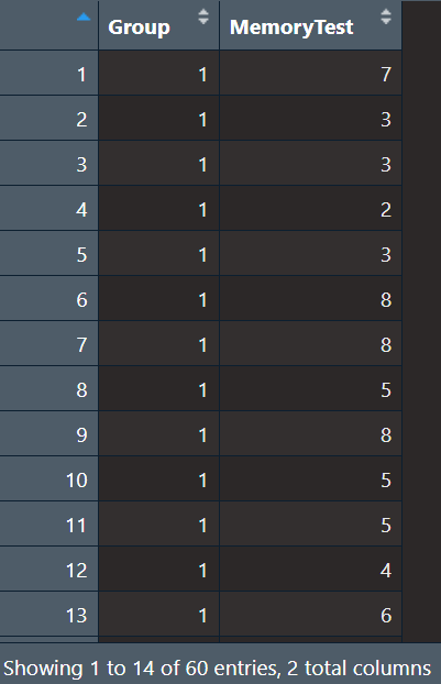
t.test(MemoryTest ~ Group, data = ch13ds1, var.equal = TRUE)
# MemoryTest ~ Group : MemoryTest(숫자)를 Group(숫자 필수x)으로 나누겠다.
# var.equal = TRUE : 같은 그룹에 대해서이므로,,
#t.test() 함수는 두 그룹 간의 평균 차이를 검정하는 함수이다.
	Two Sample t-test

data:  MemoryTest by Group
t = -0.1371, df = 58, p-value =
0.8914
alternative hypothesis: true difference in means between group 1 and group 2 is not equal to 0
95 percent confidence interval:
 -1.560009  1.360009
sample estimates:
mean in group 1 mean in group 2
       5.433333        5.533333
# 유의수준보다 값이 크다
# 따라서, 귀무가설 기각x
# 그룹별로 MemoryTest값은 평균이 같다.
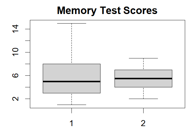
# 시각화
par(mar = c(3, 3, 2, 1)) # 마진 줄이기
memory <- boxplot(MemoryTest ~ Group, data = ch13ds1,
main = "Memory Test Scores",
xlab = "Groups", ylab = "Scores")
# main : boxplot 제목
# xlab/ylab : x축/y축 라벨
memory$stats
# 이런 정보를 확인하는 습관을 들이자. 분포 확인용
# 최솟값/1분위수/중앙값/3분위수/최댓값 정보 제시
     [,1] [,2]
[1,]    1  2.0
[2,]    3  4.0
[3,]    5  5.5
[4,]    8  7.0
[5,]   15  9.0
#leveneTest() 함수
# 그룹간 분산이 동일한지(=등분산성) 검정하는 함수
library(car)
leveneTest(MemoryTest ~ as.factor(Group), data = ch13ds1)
# as.factor(Group) : Group이 숫자값으로 되어있음.
# 범주형으로 이미 설정되어 있을 수도 있지만, 혹시 숫자로 인식하지 않게 설정하기
Levene's Test for Homogeneity of Variance (center = median)
      Df F value  Pr(>F)
group  1  3.3429 0.07264 .
      58
---
Signif. codes:
  0 ‘***’ 0.001 ‘**’ 0.01 ‘*’
  0.05 ‘.’ 0.1 ‘ ’ 1
# 유의확률이 0.07264
# 유의확률 옆의 .은 밑의 signif. codes의 '.'
# 의미는 0.05에서 0.1 사이의 값이기에,
# 0.05가 유의수준이면 유의하지 않고(즉, 귀무가설을 받아들이고),
# 0.1이 유의수준이면 유의하다(즉, 귀무가설을 기각한다).
# 유의수준이 0.1이라고 해보자.
# 그렇다면 결론은 그룹별로 분산이 동일하지 않다.
# 위 결론으로 다시 t.test를 돌리기
t.test(MemoryTest ~ Group, data = ch13ds1, var.equal = FALSE)
# var.equal = FALSE : 분산이 동일하지 않다.
# var.equal은 FALSE가 default라서 생략해도 된다.
	Welch Two Sample t-test

data:  MemoryTest by Group
t = -0.1371, df = 47.635, p-value
= 0.8915
alternative hypothesis: true difference in means between group 1 and group 2 is not equal to 0
95 percent confidence interval:
 -1.566803  1.366803
sample estimates:
mean in group 1 mean in group 2
       5.433333        5.533333
# 유의수준이 0.05라면, 유의하지 않은 결과
# 즉, 귀무가설을 유지한다.
# 분산이 다른 두 그룹별로 MemoryTest의 평균이 같다.
ch14ds1 <- read.csv("./datasets/ch14ds1.csv")
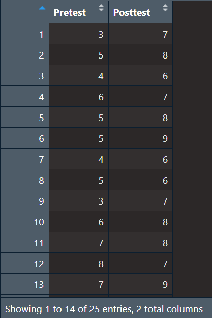
sd(ch14ds1$Pretest) # 표준편차
plot(ch14ds1$Pretest, ch14ds1$Posttest,
xlab = "Pretest", ylab = "Posttest",
main = "Pretest and Posttest Reading Achievement Scores")
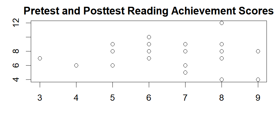
# 뚜렷한 선이 보인는 것은 아니지만, 대략적으로 양의 관계같긴 하다.
cor(ch14ds1$Pretest, ch14ds1$Posttest) # 상관계수
[1] 0.05071834
# 위 plot을 봤을때 짐작했겠지만,
# 매우 작은 양의 상관관계가 있다.
t.test(ch14ds1$Posttest, ch14ds1$Pretest, paired = TRUE,
alternative = "greater")
# paired = TRUE : 같은 사람 기준으로 비교하겠다.
# Post-Pre를 하겠다.
# alternative = "greater" : Post-Pre >=0
# 즉 단측검정
	Paired t-test

data:  ch14ds1$Posttest and ch14ds1$Pretest
t = 2.4495, df = 24,
p-value = 0.01099
alternative hypothesis: true mean difference is greater than 0
95 percent confidence interval:
 0.3618424       Inf
sample estimates:
mean difference
            1.2
# 유의수준 0.05에서는, 유의수준보다 작다.
# 따라서, 귀무가설(Post-Pre >=0) 기각.
# Post<Pre
# 전(Pre)가 후(Post)보다 크다.
# (내가 다시 봐야하는) 짧은 정리
# t-test, z-test(library(BSDA)하고 하기)가 있다. t-test는 모집단 분산 모를때 사용
# z.test에 sigma.x는 표준편
# t-test는 단일 컬럼에 대한 검정, 두개의 컬럼에 대한 검정을 할 수 있다.
# 두개의 컬럼에 대한 t- test를 할때에는 A~B(A를 B의 종류에 따라 분류하겠다)를 명시해야한다.
# var.equal = True는 등분산성인경우 조건으로 명시해야하는 식이다. default는 False
# leveneTest(library(car)하고 불러들이기)로 등분산성 검정할 수 있다.
# 수치가 범주형으로 분류되야할때 as.factor(컬럼명)을 사용한다.
# 등분산성 체크 후 t-test를 돌리는게 맞는 순서긴 하다.
# (여기에는 안 적혀있지만)유의확률/유의수준/귀무가설/대립가설, t-test의 기본 전제조건 등을 알자.
# boxplot과 plot, stats를 통해 분포를 알 수 있다. blot는 시각화, stats는 수치들로 알 수 있다.
# 아래는 기본 형식
# memory <- boxplot(MemoryTest ~ Group, data = ch13ds1,
main = "Memory Test Scores",
xlab = "Groups", ylab = "Scores")
# plot(ch14ds1$Pretest, ch14ds1$Posttest,
xlab = "Pretest", ylab = "Posttest",
main = "Pretest and Posttest Reading Achievement Scores")
# cor(ch14ds1$Pretest, ch14ds1$Posttest) 로 두 컬럼간의 상관계수를 알 수 있다.
# 같은 사람 기준 전후 비교할때에는 아래 와 같이 코드 쓴다.
# t.test(ch14ds1$Posttest, ch14ds1$Pretest, paired = TRUE,
alternative = "greater")
'Deep Learning + AI' 카테고리의 다른 글
| 데이터분석응용 in R_회귀분석 pt1 이론 (1) | 2026.04.13 |
|---|---|
| 데이터분석응용 in R_260325(update260412) (0) | 2026.04.12 |
| Generator? (0) | 2026.03.12 |
| Gemini api 관련 개념_ Context Caching (0) | 2026.03.06 |
| ERROR: No matching distribution found for torch==2.1.0 해결법 (0) | 2025.08.15 |


